Background
This was inspired by Paul Harrison’s (pfh’s) 2021 post, We’ve been doing k-means wrong for more than half a century. Pfh found that the K-means algorithm in his R package put too many clusters in dense areas, resulting in worse fits compared with just cutting a Ward clustering at height (k).
tl;dr
I re-implemented much of pfh’s notebook in Python, and found that Scikit-learn did just fine with k-means++ init, but reproduced the problem using naive init (random restarts). Cross-checking with flexclust, he decided the problem was a bug in the LICORS implementation of k-means++.
Upshot: use either Ward clustering or k-means++ to choose initial clusters. In Python you’re fine with Scikit-learn’s default. But curiously the Kward here ran somewhat faster.
Update Nov-2022: I just searched for the LICORS bug. LICORS hasn’t been maintained since 2013, but it’s popular in part for its implementation of kmeanspp , compared to the default (naive) kmeans in R’s stats package. However, it had a serious bug in the distance matrix computation reported by Bernd Fritzke in Nov. 2021 that likely accounts for the behavior Paul noticed. Apparently fixing that drastically improved its performance.
I’ve just created a pull-request to the LICORS package with that fix. It appears the buggy code was copied verbatim into the motifcluster package. I’ve added a pull request there.
Summarizing pfh
- k-means tries to minimise sum-of-squared distances of points to clusters
- The usual Lloyd’s algorithm is fast, but gets stuck near the initial guess.
- Initializing by random choice distributes clusters proportional to point density.
- But cluster centers should be more spread out, roughly as density to the power $\frac{d}{d+2}$, where $d$ is number of dimensions.
- k-means++ and Ward both seem to do this.
- In one dimension, fast exact solutions are possible. R:Ckmeans.1d.dp, Python:ckwrap, ckmeans
| “ | I believe k-means is an essential tool for summarizing data. It is not simply “clustering”, it is an approximation that provides good coverage of a whole dataset by neither overly concentrating on the most dense regions nor focussing too much on extremes. Maybe this is something our society needs more of. Anyway, we should get it right. ~pfh |
References
Citation for fastcluster:
Daniel Müllner, fastcluster:Fast Hierarchical, Agglomerative Clustering Routines for R and Python, Journal of Statistical Software 53 (2013), no. 9, 1–18, URL http://www.jstatsoft.org/v53/i09/
Speed depends on many things.
- Note the up-to-1000x improvements in this 2018 discussion of sklearn’s k-means by using Cython, OpenMP, and well-vectorized code. (The ticket is closed with a [MRG] note, so may have been incorporated already.)
- And this 2020 post says Facebook’s
faisslibrary is 8x faster and 27x more accurate thansklearn, at least on larger datasets like MNIST. - Or a 2017 post for CFXKMeans promising 78x speedup – though note sklearn may have gotten much faster since then.
Test Times & Scores
I’ll omit the code running the tests. Defined null_fit() , do_fits(), do_splice(),
functions to run fits and then combine results into a dataframe.
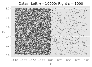
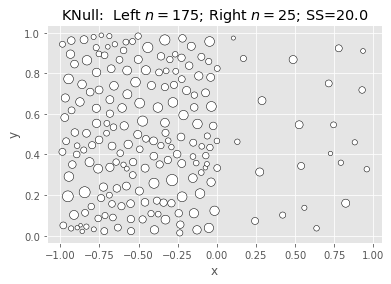
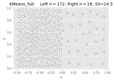
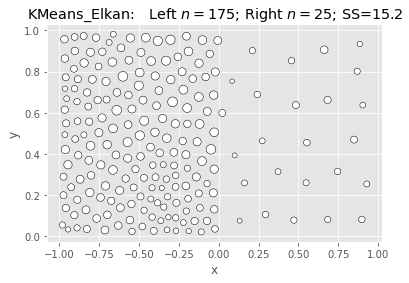
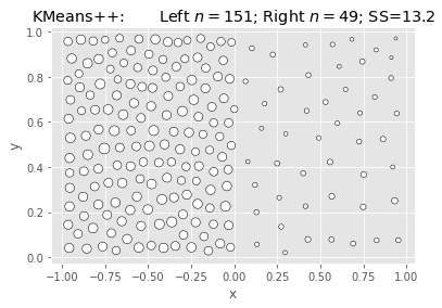
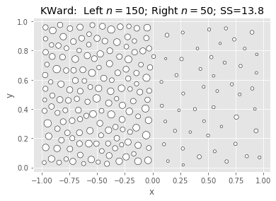
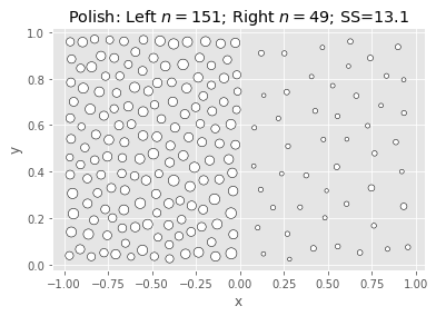
Borrowing an example from pfh, we will generate two squares of uniform density, the first with 10K points and the second with 1K, and find $k=200$ means. Because the points have a ratio of 10:1, we expect the ideal #clusters to be split $\sqrt{10}:1$.
| Name | Score | Wall Time[s] | CPU Time[s] | |
|---|---|---|---|---|
| 0 | KNull | 20.008466 | 0.027320 | 0.257709 |
| 1 | KMeans_full | 14.536896 | 0.616821 | 6.964919 |
| 2 | KMeans_Elkan | 15.171172 | 4.809588 | 69.661552 |
| 3 | KMeans++ | 13.185790 | 4.672390 | 68.037351 |
| 4 | KWard | 13.836546 | 1.694548 | 4.551085 |
| 5 | Polish | 13.108796 | 0.176962 | 2.568561 |
Python
We see the same thing using vanilla k-means (random restarts), but the default k-means++ init overcomes it.
The Data:
SciKit KMeans: Null & Full (Naive init):
|
|
SciKit KMeans: Elkan & Kmeans++:
|
|
Ward & Polish:
|
|
More data: vary $n1, k$
What we’re seeing above is that Ward is fast and nearly as good, but not better.
Let’s collect multiple samples, varying $k$ and $n1$ as we go.
| Name | Score | Wall Time[s] | CPU Time[s] | k | n1 | |
|---|---|---|---|---|---|---|
| 0 | KNull | 10.643565 | 0.001678 | 0.002181 | 5 | 10 |
| 1 | KMeans_full | 4.766947 | 0.010092 | 0.010386 | 5 | 10 |
| 2 | KMeans_Elkan | 4.766947 | 0.022314 | 0.022360 | 5 | 10 |
| 3 | KMeans++ | 4.766947 | 0.027672 | 0.027654 | 5 | 10 |
| 4 | KWard | 5.108086 | 0.008825 | 0.009259 | 5 | 10 |
| ... | ... | ... | ... | ... | ... | ... |
| 475 | KMeans_full | 14.737051 | 0.546886 | 6.635604 | 200 | 1000 |
| 476 | KMeans_Elkan | 14.452111 | 6.075230 | 87.329714 | 200 | 1000 |
| 477 | KMeans++ | 13.112620 | 5.592246 | 78.233175 | 200 | 1000 |
| 478 | KWard | 13.729485 | 1.953153 | 4.668957 | 200 | 1000 |
| 479 | Polish | 13.091032 | 0.144555 | 2.160262 | 200 | 1000 |
480 rows × 6 columns
Plot Scores
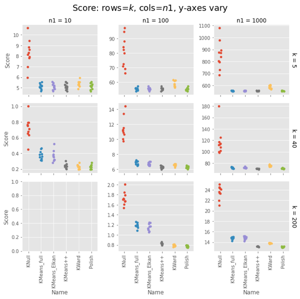
We will see that KWard+Polish is often competitive on score, but seldom better.
- rows = $k$
- columns = $n1$ (with $n2 = 10 \times n1$
Pfh’s example was for $n1 = 1000$ and $k = 200$.
Plot CPU Times
Remember that polish() happens after the Ward clustering, so you should really add those two columns. But in most cases it’s on the order of the KNull.
Even with the polish step, Ward is generally faster, often much faster. The first two has curious exceptions for $n1 = 100, 1000$. I’m tempted to call that setup overhead, except it’s not there for $n1 = 10$, and the charts have different orders of magnitude for the $y$ axis.
Note that the wall-time differences are less extreme, as KMeans() uses concurrent processes. (That helps the polish() step as well, but it usually has few iterations.)
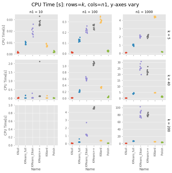
Fair enough: On uniform random data, Ward is as fast as naive K-means and as good as a k-means++ init.
How does it do on data it was designed for? Let’s make some blobs and re-run.
Test with Real Clusters
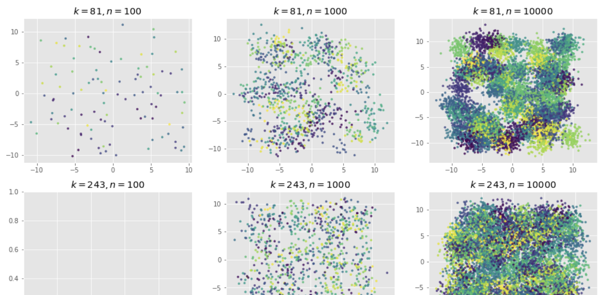
OK, so that’s how it performs if we’re just quanitizing uniform random noise. What about when the data has real clusters? Saw blob generation on the faiss example post.
Preview of some of the data we’re generating:
| Name | Score | Wall Time[s] | CPU Time[s] | k | n1 | |
|---|---|---|---|---|---|---|
| 0 | KNull | 448.832176 | 0.001025 | 0.001025 | 5 | 100 |
| 1 | KMeans_full | 183.422464 | 0.007367 | 0.007343 | 5 | 100 |
| 2 | KMeans_Elkan | 183.422464 | 0.010636 | 0.010637 | 5 | 100 |
| 3 | KMeans++ | 183.422464 | 0.020496 | 0.020731 | 5 | 100 |
| 4 | KWard | 183.422464 | 0.006334 | 0.006710 | 5 | 100 |
| ... | ... | ... | ... | ... | ... | ... |
| 235 | KMeans_full | 3613.805107 | 0.446731 | 5.400928 | 200 | 10000 |
| 236 | KMeans_Elkan | 3604.162116 | 4.658532 | 68.597281 | 200 | 10000 |
| 237 | KMeans++ | 3525.459731 | 4.840202 | 71.138150 | 200 | 10000 |
| 238 | KWard | 3665.501244 | 1.791814 | 4.648277 | 200 | 10000 |
| 239 | Polish | 3499.884487 | 0.144633 | 2.141082 | 200 | 10000 |
240 rows × 6 columns
Scores
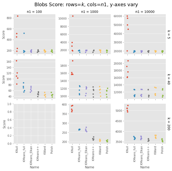
Ward and Polish score on par with KMeans++. For some combinations of $n1$ and $k$ the other algorithms are also on par, but for some they do notably worse.
CPU Times
Ward is constant for a given $n1$, about 4-5s for $n1 = 10,000$. KMeans gets surprisingly slow as $k$ increases, taking 75s vs. Ward’s 4-5s for $k=200$. Even more surprising, Elkan is uniformly slower than full. This could be intepreted vs. compiled, but needs looking into.
The basic result holds.
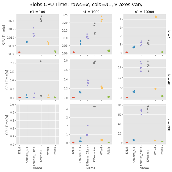
Strangely, Elkan is actually slower than the old EM algorithm, despite having well-organized blobs where the triangle inequality was supposed to help.
Conclusion
On both uniform random data and blob data, KWard+Polish scores like k-means++ while running as fast as vanilla k-means (random restarts).
In uniform data, the polish step seems to be required to match k-means++. In blobs, you can pretty much stop after the initial Ward.
Surprisingly, for sklearn the EM algorithm (algorithm='full') is faster than the default Elkan.
Appendix: the Classes
We defined two classes for the tests:
- KNull - Pick $k$ data points at at random and call that your answer.
- KWard - A drop-in replacement for Scikit-Learn’s KMeans, but uses Ward hierarchical clustering, but at height $k$.
We call the fastcluster package for the actual Ward clustering, and provide a .polish() method to do a few of the usual EM iterations to polish the result.
It gives results comparable to the default k-means++ init, but (oddly) was notably faster for large $k$. This is probably just interpreted versus compiled, but needs some attention. Ward is $O(n^2)$ while k-means++ is $O(kn)$, but Ward was running in 4-5s while scikit-learn’s kmeans ++ was taking notably longer for $k≥10$. For $k=200$ it took 75s. (!!)
The classes are really a means to an end here. The post is probably most interesting as:
- identifying a bug in an R package,
- learning a bit more about what makes K-means solutions good
- finding an odd slowness in scikit-learn’s k-means.
KNull Class
KNull just choses $k$ points at random from $X$. We could write that from scratch, but it’s equivalent to calling KMeans with 1 init and 1 iteration. (Besides, I was making a subclassing mistake in KWard, and this minimal subclass let me track it down.)
class KNull(KMeans):
    """KMeans with only 1 iteration: pick $k$ points from $X$."""
    def __init__(self,
                 n_clusters: int=3,
                 random_state: RandLike=None):
        """Initialize w/1 init, 1 iter."""
        super().__init__(n_clusters,
                        init="random",
                        n_init=1,
                        max_iter=1,
                        random_state=random_state)
Aside: A quick test confirms .inertia_ stores the training .score(mat). Good because it runs about 45x faster.
KWard Class
We make this a subclass of KMeans replacing the fit() method with a call to fastcluster.linkage_vector(X, method='ward') followed by cut_tree(k) to get the initial clusters, and a new polish() method that calls regular KMeans starting from the Ward clusters, and running up to 100 iterations, polishing the fit. (We could put polish() into fit() but this is clearer for testing.
Note: The _vector is a memory-saving variant. The Python fastcluster.linkage*() functions are equivalent to the R fastcluster.hclust*() functions.
class KWard(KMeans):
    """KMeans but use Ward algorithm to find the clusters.

    See KMeans for full docs on inherited params.

    Parameters
    -----------
    These work as in KMeans:
        n_clusters : int, default=8
        verbose : int, default=0
        random_state : int, RandomState instance, default=None

    THESE ARE IGNORED:
        init, n_init, max_iter, tol
        copy_x, n_jobs, algorithm


    Attributes
    -----------
    algorithm : "KWard"

    Else, populated as per KMeans:
        cluster_centers_
        labels_
        inertia_
        n_iter_ ????

    Notes
    -------
    Ward hierarchical clustering repeatedly joins the two most similar points. We then cut the
    resulting tree at height $k$.  We use the fast O(n^2) implementation in fastcluster.

    """
    def __init__(self, n_clusters: int=8, *,
                 verbose: int=0, random_state=None):
        super().__init__(n_clusters,
                         verbose = verbose,
                         random_state = random_state)
        self.algorithm = "KWard" # TODO: Breaks _check_params()
        self.polished_ = False

    def fit(self, X: np.array, y=None, sample_weight=None):
        """Find K-means cluster centers using Ward clustering.

        Set .labels_, .cluster_centers_, .inertia_.
        Set .polished_ = False.

        Parameters
        ----------
        X : {array-like, sparse matrix} of shape (n_samples, n_features)
            Passed to fc.linkage_vector.

        y : Ignored

        sample_weight : Ignored
            TODO: does fc support weights?

        """
        # TODO - add/improve the validation/check steps
        X = self._validate_data(X, accept_sparse='csr',
                               dtype=[np.float64, np.float32],
                               order='C', copy=self.copy_x,
                               accept_large_sparse=False)

        # Do the clustering. Use pandas for easy add_col, groupby.
        hc = fc.linkage_vector(X, method="ward")
        dfX = pd.DataFrame(X)
        dfX['cluster'] = cut_tree(hc, n_clusters=self.n_clusters)

        # Calculate centers, labels, inertia
        _ = dfX.groupby('cluster').mean().to_numpy()
        self.cluster_centers_ = np.ascontiguousarray(_)
        self.labels_ = dfX['cluster']
        self.inertia_ = -self.score(X)

        # Return the raw Ward clustering assignment
        self.polished_ = False
        return self

    def polish(self, X, max_iter: int=100):
        """Use KMeans to polish the Ward centers. Modifies self!"""
        if self.polished_:
            print("Already polished. Run .fit() to reset.")
            return self

        # Do a few iterations
        ans = KMeans(self.n_clusters, n_init=1, max_iter=max_iter,
                     init=self.cluster_centers_)\
                .fit(X)

        # How far did we move?
        𝛥c = np.linalg.norm(self.cluster_centers_ - ans.cluster_centers_)
        𝛥s = self.inertia_ - ans.inertia_
        print(f"   Centers moved by: {𝛥c:8.1f};\n"
              f"  Score improved by: {𝛥s:8.1f} (>0 good).")
        self.labels_ = ans.labels_
        self.inertia_ = ans.inertia_
        self.cluster_centers_ = ans.cluster_centers_
        self.polished_ = True
        return self
Usage: KWard(k).fit(X) or KWard(k).fit(X).polish(X).