i’m not sure what this says about me other than gosh it was a nice day…

i’m not sure what this says about me other than gosh it was a nice day…
Loved this whimsy.

I had a lovely hour last night chasing the Orion Nebula with my 16yo at a local soccer field with our new scope. We enjoyed seeing more things every time we swapped lenses, and describing what we saw. Her eyes are better, so she figured out first that the one blurry star in the wide view was actually a tiny trapezoid of four stars very close together. At higher power they separated quite nicely, and we began to see the contours of the nebula. Not bad for the local soccer field, a crescent moon straight overhead, and some high clouds. Plus, memories.

The scope is a used Telescopics 8" reflector from the 1980s in a pretty wooden cradle on a Dobsonian mount. The mirror seems to be really good. (Photo by Bob Parks from the club sale.)
I see crypto as dystopian by design, but Daniel Meissler’s re-imagining at least lets me glimpse why it might have general appeal.
Take a multi-player world like MineCraft where people create amazing fantastic, complicated things. That seems to be working fine right now, but it seems a really creative builder or gamer needs YouTube or Patreon or a side job. Meissler:
| ❝ | So an example would be a user signing up, creating a cool city or island in a game, standing up a government, creating really cool magic items, etc., and making money when people decide to come there and spend time (because they like how the system works). |
I’m not sure this is better but it’s not obviously bad. It has the benefits and flaws of how we build valuable things & experiences in the real world.
And I’m not sure it needs blockchain – didn’t Steam already do this a decade ago without crypto?
But at least he sketches why there might a coordination problem to solve, rather than a cool hammer hunting nails.
| ❝ | If you find you always agree with the liberal or conservative party, then that is your true religion. |
Today it was this 2016 Jacobs piece I found from his tribute to Paul Farmer.
I have at times been in groups of people who know and respect the work of Care Net, but if in those contexts I mention my admiration for the work of Paul Farmer and Partners in Health, I am liable to get some suspicious looks. …
In other groups, people join enthusiastically in my praise for Paul Farmer — but become nervous when I mention my admiration for Care Net. …
And yet both Partners in Health and Care Net are pursuing the Biblical mandate to care for the weakest and most helpless among us. In so many ways they are doing the same work, and even are dedicated to the same goal — the preservation and healing of the lives of people made in the image of God. Why must we see them in opposition to each other?
I signed into µ.blog to bookmark some tech piece and found instead that Paul Farmer has died.
| ❝ | If you must write about us, at least give a damn about us, |
Not just “if you write, give a damn”, but about us. This is about community and relationships. She’s tempted to outrage, but she lives there, and “outrage is where relationships go to die.”
Outrage doesn’t get curious about why. It mutes the Principle of Charity. It often reacts to imagined motive more than act. Witness Colin Kaepernick taking a knee.
To be sure, there is plenty of anti-Semitism about, and Maus is charismatic megafauna, worthy of defense. But,
The meeting minutes suggest that their objections to Art Spiegelman’s _Maus_ series had less to do with the subject matter and more to do with a purity narrative _that never seems to die_, no matter the zip code.In a response [Margaret Renki agrees](https://www.nytimes.com/2022/02/07/opinion/culture/maus-tennessee-book-bans.html), wryly noting:
Around here, antisemitism tends to take far more flagrant forms,
The minutes show a board mostly committed to teaching the Holocaust, but deeply uncomfortable making main unit text contain, as Renki summarizes, “profanity, sexuality, violence and… a suicide scene.” They wanted to just fully redact eight words and an image, but were advised that might exceed “fair use”.
That’s like restricting Alice in Wonderland for promoting poison, but as Renki notes, purity culture is universal: my demographic doesn’t mind literary profanity, but we have put two prize-winning classics on the Top 10 Banned Books list, for violating other norms.
Back to Kimball Coe:
| ❝ |
I’ve got to be on the side of holding that together. : If you want to signal to the world that you’re on the side of solutions and repair, then write or tweet as a repairer of the breach. |
This seems so very Catholic:
| ❝ | But as Bell’s wise documentary also makes clear, there wasn’t really one Bill Cosby and another secret one. There isn’t a good Cosby and a bad Cosby, whom we can store in different mental compartments. There is just Bill Cosby, about whom we didn’t know enough and now know dreadfully more. In the end, Dr. Jekyll and Mr. Hyde are always the same guy. |
Also worth reading, Will Wheaton’s response to a question about Joss Whedon.
Python Anti-Pattern: Default Mutable Arguments
@SourceryAI found a bad habit I didn’t know I had: def f(names: list=[]):. This would be nearly impossible to debug.
| ❝ |
When we’re good at participatory sense-making, we can become societies that support each member, where we can each bring as much of ourselves as we like. ...
On our software teams, we have to get good at participatory sense-making to make strong, consistent software. To do this, … We get better at personing. …We get farther together; that frustration has value. ~Jessica Kerr |
Software pushes us to get better as people, on her blog Jessitron.
| ❝ |
Wouldn’t it be nice if we could train scientists to be communicators and be personal like this with audiences without needing somebody like me standing beside them, helping it happen?
~ Alan Alda |
From a recent AAAS member spotlight on Alan Alda. It continues:
Today, the Alda Center has thus far trained some 20,000 scientists and medical professionals around the world to share science in a clear, engaging and accessible manner.
Periodically a song from “The Greatest Showman” is on my mental background music.
I just noticed my brain had substituted for “anthem”:
 Let this promise in me start
 Like an anvil in my heart
 ...
🤔
| ❝ | Debugging is twice as hard as writing the code in the first place. Therefore, if you write the code as cleverly as possible, you are, by definition, not smart enough to debug it. ~Brian Kernighan |
Bookmark: Alan Jacobs excerpting a recent Rowan Williams essay in The New Statesman. Education, Science, and Humanities.
Dear Self: Remember periodically to reread Dorothy Bishop’s (@DeevyBee) recent reflection on humility and choosing battles, “Why I am not engaging with the Reading Wars”.
Huh! Quite OK Image compression provides a simple fast algorithm and format that seems to benchmark well. Encodes the next pixel as either run-length, small diffs, or recently-seen.
Headlines about the death of theory are philosopher clickbait. Fortunately Laura Spinney’s article is more self-aware than the headline:
| ❝ | But Anderson’s [2008] prediction of the end of theory looks to have been premature – or maybe his thesis was itself an oversimplification. There are several reasons why theory refuses to die, despite the successes of such theory-free prediction engines as Facebook and AlphaFold. All are illuminating, because they force us to ask: what’s the best way to acquire knowledge and where does science go from here? |
(Note: Laura Spinney also wrote Pale Rider, a history of the 1918 flu.)
Forget Facebook for a moment. Image classification is the undisputed success of black-box AI: we don’t know how to write a program to recognize cats, but we can train a neural net on lots of picture and “automate the ineffable”.
But we’ve had theory-less ways to recognize cat images for millions of years. Heck, we have recorded images of cats from thousands of years ago. Automating the ineffable, in Kozyrkov’s lovely phrase, is unspeakably cool, but it has no bearing on the death of theory. It just lets machines do theory-free what we’ve been doing theory-free already.
The problem with black boxes is supposedly that we don’t understand what they’re doing. Hence DARPA’s “Third Wave” of Explainable AI. Kozyrkov thinks testing is better than explaining - after all we trust humans and they can’t explain what they’re doing.
I’m more with DARPA than Kozyrkov here: explainable is important because it tells us how to anticipate failure. We trust inexplicable humans because we basically understand their failure modes. We’re limited, but not fragile.
But theory doesn’t mean understanding anyway. That cat got out of the bag with quantum mechanics. Ahem.
Apparently the whole of quantum theory follows from startlingly simple assumptions about information. That makes for a fascinating new Argument from Design, with the twist that the universe was designed for non-humans, because humans neither grasp the theory nor the world it describes. Most of us don’t understand quantum. Well maybe Feynman, though even he suggested he might not really understand.
Though Feynman and others seem happy to be instrumentalist about theory. Maybe derivability is enough. It is a kind of understanding, and we might grant that to quantum.
But then why not grant it to black-box AI? Just because the final thing is a pile of linear algebra rather than a few differential equations?
I think it was Wheeler or Penrose – one of those types anyway – who imagined we met clearly advanced aliens who also seemed to have answered most of our open mathematical questions.
And then imagined our disappointment when we discovered that their highly practical proofs amounted to using fast computers to show they held for all numbers tried so far. However large that bound was, we should be rightly disappointed by their lack of ambition and rigor.
Theory-free is science-free. A colleague (Richard de Rozario) opined that “theory-free science” is a category error. It confuses science with prediction, when science is also the framework where we test predictions, and the error-correction system for generating theories.
Three examples from the article:
Certainly. Since the 1970s when Meehl showed that simple linear regressions could outpredict psychiatrists, clinicians, and other professionals. In later work he showed they could do that even if the parameters were random.
So beating these humans isn’t prediction trumping theory. It’s just showing disciplines with really bad theory.
I admire Tom Griffiths, and any work he does. He’s one of the top cognitive scientists around, and using neural nets to probe the gaps in prospect theory is clever; whether it yield epicycles or breakthroughs it should advance the field.
He’s right that more data means you can support more epicycles. But basic insights Wallace’s MML remain: if the sum of your theory + data is not smaller than the data, you don’t have an explanation.
AlphaFold’s jumping-off point was the ability of human gamers to out-fold traditional models. The gamers intuitively discovered patterns – though they couldn’t fully articulate them. So this was just another case of automating the ineffable.
But the deep nets that do this are still fragile – they fail in surprising ways that humans don’t, and they are subject to bizarre hacks, because their ineffable theory just isn’t strong enough. Not yet anyway.
So we see that while half of success of Deep Nets is Moore’s law and Thank God for Gamers, the other half is tricks to regularize the model.
That is, to reduce its flexibility.
I daresay, to push it towards theory.
Marvel’s The Eternals is not my favorite, but I’m liking it a bit more after Film Theory linked the plot to Thanos – and gave the first plausible Thanos redemption I’ve heard.
Deborah Mayo has a new post on Model Testing and p-values vs. posteriors.
I haven’t read Bickel, but now want to. So thanks for the alert.
Fisher is surely right about facetiously adopting extreme priors – a “million to one” prior shouldn’t happen without some equivalent of a million experiences, and a “model check” on the priors makes sense if you want more than a hypothetical.
But surely, his paragraph about “not capable of finding expression in any calculation” is rhetorical fluff amounting you “you have the wrong model”. If priors are plucked from the air, they can be airily dismissed.
On this note I find his switch to parapsychology puzzling (follow her link to pp. 42-44). His Pleiades example shows that their unlikely clustering makes it hard to accept randomness despite the posterior odds still favoring randomness by 30:1. I think he is arguing that the sheer weight of evidence makes us doubt our prior assumption. And rightly so – how confident were we of that million:1 guesstimate anyway?
But his parapsychology example seems to make the opposite point. Here we (correctly) stick to our prior skepticism, and explain away the surprising results as fabrications, mistakes, etc. Here our prior is informed by many things including a century of failed parapsychology experiments – or more precisely a pattern of promising results falling apart under scrutiny. Like prospects for a new cancer drug, we expect it to let us down.
I like to think that “simple” Bayesian inference over all computable models wouldn’t suffer this problem, because all model classes are included. This being intractable, we typically calculate posteriors inside small convenient model families. If things look very wrong, hopefully we remember we may just have the wrong model. Though probably not before adding some epicycles.
[swapped first two paragraphs; tweaks for clarity]
So this Philosophy Stackexchange answer by bobflux has me thinking, even as I’m about to get my booster shot. It’s long, but well-argued.
Intuition: Antibiotic resistance means you must finish your whole prescription so you kill the whole population, instead of just selecting for resistant ones. There is a similar concern with leaky vaccines.
My short summary, in table form plus three notes:
| Sterilizing (Measles vax) | Leaky (Covid vax) | |
|---|---|---|
| Contagious (e.g. Measles) | Vaccinate lots: balance side-effects & infection. No evolution. | More vax ➛ more resistant. 3 paths: 1) Dengue: ☠️ vaxed; 2) Marek: ☠️ unvaxed; 3) common cold |
| Non-Contagious (e.g. Tetanus) | Get if you want. Little impact on others. | –NA– |
Expanding on those three paths:
Dengue vax caused antibody-dependent enhancement (ADE), where the vaccine increased viral load, making Dengue more deadly to the vaxxed. Ouch.
Marek vax in chickens extends infections of “strains otherwise too lethal to persist”. What used to paralyze and kill old birds is now 100% lethal even to young. All must be vaxxed, and will be carriers.
Common cold: Those with mild case go out and about, spreading mild variants and immunities. Those very sick stay home and spread less. Utilitarians have a moral obligation to host Covid Parties.
~End Summary~
I’m happily on the annual-flu-shot train, esp. on the hope that by the time I’m 70 and need it, my system will have seen a lot of variants. Also, I haven’t heard any worries about breeding more resistant flu. I’ve been assuming for awhile that COVID would follow the common-cold path of becoming prevalent and mild, at worst flu-like with annual vaccines. And given that it’s impossible to avoid exposure, it seems better to get side effects of the spike protein rather than infection effects of the live virus.
Now twice in the last week I’ve come across the 2015 paper about the Marek experiment and am thinking about the evolutionary dynamics, and monocultures. How to tell what path we are on? When is it better to Stoically accept the current infections to spare future generations?
More immediately, should I go through with the booster shot? (Given it’s scheduled for tomorrow, that’s the default and most likely outcome. But I am wondering. )
Discovered my new favorite Thanksgiving poem/prayer, from Malcom Guite:
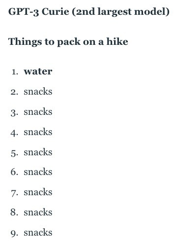
Janelle Shane asks GPT-3 what else besides water to bring on a hike. More here
Dashboards are the opposite. They’re often data, looking for a problem.
Like so many of his interviews, this with McChrystal looks fascinating.
I found the beginning of the Srinivasan interview painful, but it improved later. I enjoyed Sullivan’s take on UK vs US. And I’m halfway through the rivetting discussion with Tufecki on COVID-19 response.
Good essay. I did not know the tragic Aaron Swartz story.
This struck me too:
Perhaps the KGB would have enjoyed a better reputation if they had merely charged astronomical sums for copies of Solzhenitsyn.