~NYT on [Emmanual Todd & the Decline of the West](https://www.nytimes.com/2024/03/09/opinion/emmanuel-todd-decline-west.html)

Thoughts

The US has infant and maternal mortality problems, but is it this bad, or is it just Russia finally catching up?

• The CIA World Fact Book estimates 2023 Russia still behind at 6.6 infant deaths per thousand live births, versus 5.1 for the US. For comparison, it estimates 35 European countries are below 5 per thousand, and the US is on par with Poland.

• In contrast, Macrotrends data says Russia has edged ahead at 4.8, while it rates the US worse at 5.5. (US and RU data here.) That’s in line with Todd’s US number, and they claim to source from the UN World Population Prospects, so I’ll presume some overlap there. I don’t know the sources myself.

But here’s a combined trend using Macrotrend’s data, from 1960-2024 (omitting Russia’s disastrous 1950s). Even this data has the US slowly improving, so the story is Russia catching up.

Possibly relevant: birth rates are similar at 11 & 12 per thousand (Macrotrends).

Either way, Russia is close to the US now, and I’m surprised – my impressions were outdated. But this graph doesn’t seem cause for concern about the US. Comparison to peer democracies might. I’d have to read Todd’s book for the argument.

Other striking thoughts:

A specialist in the anthropology of families, Mr. Todd warns that a lot of the values Americans are currently spreading are less universal than Americans think.

Which thought continues:

In a similar way, during the Cold War, the Soviet Union’s official atheism was a deal-breaker for many people who might otherwise have been well disposed toward Communism.

And despite the US haing ~2.5x Russia’s population (per US Census):

Mr. Todd calculates that the United States produces fewer engineers than Russia does, not just per capita but in absolute numbers.

Though this may reflect his values for what counts as productive (my emphasis):

It is experiencing an “internal brain drain,” as its young people drift from demanding, high-skill, high-value-added occupations to law, finance and various occupations that merely transfer value around the economy and in some cases may even destroy it. (He asks us to consider the ravages of the opioid industry, for instance.)

A Berkeley Computer Science lab just uploaded “Approaching Human-Level Forecasting with Language Models” to arXiv DOI:10.48550/arXiv.2402.18563. My take:

There were three things that helped: Study, Scale, and Search, but the greatest of these is Search.

Halawi et al replicated earlier results that off-the-shelf LLMs can’t forecast, then showed how to make them better. Quickly:

• A coin toss gets a squared error score of 0.25.
• Off-the-shelf LLMs are nearly that bad.
• Except GPT-4 that got 0.208.
• With web search and fine tuning, the best LLMs got down to 0.179.
• The (human) crowd average was 0.149.

Adding news search and fine tuning, the LLMs were decent (Brier .179), and well-calibrated. Not nearly as good as the crowd (.149), but probably (I’m guessing) better than the median forecaster – most of crowd accuracy is usually carried by the top few %. I’m surprised by the calibration.

Search

By far the biggest gain was adding Info-Retrieval (Brier .206 -> .186), especially when it found at least 5 relevant articles.

With respect to retrieval, our system nears the performance of the crowd when there are at least 5 relevant articles. We further observe that as the number of articles increases, our Brier score improves and surpasses the crowd’s (Figure 4a). Intuitively, our system relies on high-quality retrieval, and when conditioned on more articles, it performs better.

Note: they worked to avoid information leakage. The test set only used questions published after the models' cutoff date, and they did sanity checks to ensure the model didn’t already know events after the cutoff date (and did know events before it!). New retrieval used APIs that allowed cutoff dates, so they could simulate more information becoming available during the life of the question. Retrieval dates were sampled based on advertised question closing date, not actual resolution.

Study:

Fine-tuning the model improved versus baseline: (.186 -> .179) for the full system, with variants at 0.181-0.183. If I understand correctly, it was trained on model forecasts of training data which had outperformed the crowd but not by too much, to mitigate overconfidence.

That last adjustment – good but not too good – suggests there are still a lot of judgmental knobs to twiddle, risking a garden of forking paths. However, assuming no actual flaws like information leakage, the paper stands as an existence proof of decent forecasting, though not a representative sample of what replication-of-method would find.

Scale:

GPT4 did a little better than GPT3.5. (.179 vs .182). And a lot better than lunchbox models like Llama-2.

But it’s not just scale, as you can see below: Llama’s 13B model outperforms its 70B, by a lot. Maybe sophistication would be a better word, but that’s too many syllables for a slogan.

Thoughts

Calibration: was surprisingly good. Some of that probably comes from the careful selection of forecasts to fine-tune from, and some likely from the crowd-within style setup where the model forecast is the trimmed mean from at least 16 different forecasts it generated for the question. [Update: the [Schoenegger et al] paper (also this week) ensembled 12 different LLMs and got worse calibration. Fine tuning has my vote now.]

Forking Paths: They did a hyperparameter search to optimize system configuration like the the choice of aggregation function (trimmed mean), as well as retrieval and prompting strategies. This bothers me less than it might because (1) adding good article retrieval matters more than all the other steps; (2) hyperparameter search can itself be specified and replicated (though I bet the choice of good-but-not-great for training forecasts was ad hoc), and (3) the paper is an existence proof.

Quality: It’s about 20% worse than the crowd forecast. I would like to know where it forms in crowd %ile. However, it’s different enough from the crowd that mixing them at 4:1 (crowd:model) improved the aggregate.

They note the system had biggest Brier gains when the crowd was guessing near 0.5, but I’m unimpressed. (1) this seems of little practical importance, especially if those questions really are uncertain, (2) it’s still only taking Brier of .24 -> .237, nothing to write home about, and (3) it’s too post-hoc, drawing the target after taking the shots.

Overall: A surprising amount of forecasting is nowcasting, and this is something LLMs with good search and inference could indeed get good at. At minimum they could do the initial sweep on a question, or set better priors. I would imagine that marrying LLMs with Argument Mapping could improve things even more.

This paper looks like a good start.

Linda McIver and Cory Doctorow do not buy the AI hype.

McIver ChatGPT is an evolutionary dead end:

As I have noted in the past, these systems are not intelligent. They do not think. They do not understand language. They literally choose a statistically likely next word, using the vast amounts of text they have cheerfully stolen from the internet as their source.

Doctorow’s Autocomplete Worshippers:

AI has all the hallmarks of a classic pump-and-dump, starting with terminology. AI isn’t “artificial” and it’s not “intelligent.” “Machine learning” doesn’t learn. On this week’s Trashfuture podcast, they made an excellent (and profane and hilarious) case that ChatGPT is best understood as a sophisticated form of autocomplete – not our new robot overlord.

Not so fast. First, AI systems do understand text, though not the real-world referents. Although LLMs were trained by choosing the most likely word, they do more. Representations matter. How you choose the most likely word matters. A very large word frequency table could predict the most likely word, but it couldn’t do novel word algebra (king - man + woman = ___) or any of the other things that LLMs do.

Second, McIver and Doctorow trade on their expertise to make their debunking claim: we understand AI. But that won’t do. As David Mandel notes in a recent preprint AI Risk is the only existential risk where the experts in the field rate it riskier than informed outsiders.

Google’s Peter Norvig clearly understands AI. And he and colleagues argue they’re already general, if limited:

Artificial General Intelligence (AGI) means many different things to different people, but the most important parts of it have already been achieved by the current generation of advanced AI large language models such as ChatGPT, Bard, LLaMA and Claude. …today’s frontier models perform competently even on novel tasks they were not trained for, crossing a threshold that previous generations of AI and supervised deep learning systems never managed. Decades from now, they will be recognized as the first true examples of AGI, just as the 1945 ENIAC is now recognized as the first true general-purpose electronic computer.

That doesn’t mean he’s right, only that knowing how LLMs work doesn’t automatically dispel claims.

Meta’s Yann LeCun clearly understands AI. He sides with McIver & Doctorow that AI is dumber than cats, and argues there’s a regulatory-capture game going on. (Meta wants more openness, FYI.)

Demands to police AI stemmed from the “superiority complex” of some of the leading tech companies that argued that only they could be trusted to develop AI safely, LeCun said. “I think that’s incredibly arrogant. And I think the exact opposite,” he said in an interview for the FT’s forthcoming Tech Tonic podcast series.

Regulating leading-edge AI models today would be like regulating the jet airline industry in 1925 when such aeroplanes had not even been invented, he said. “The debate on existential risk is very premature until we have a design for a system that can even rival a cat in terms of learning capabilities, which we don’t have at the moment,” he said.

Could a system be dumber than cats and still general?

McIver again:

There is no viable path from this statistical threshing machine to an intelligent system. You cannot refine statistical plausibility into independent thought. You can only refine it into increased plausibility.

I don’t think McIver was trying to spell out the argument in that short post, but as stated this begs the question. Perhaps you can’t get life from dead matter. Perhaps you can. The argument cannot be, “It can’t be intelligent if I understand the parts”.

Doctorow refers to Ted Chiang’s “instant classic”, ChatGPT Is a Blurry JPEG of the Web

[AI] hallucinations are compression artifacts, but—like the incorrect labels generated by the Xerox photocopier—they are plausible enough that identifying them requires comparing them against the originals, which in this case means either the Web or our own knowledge of the world.

I think that does a good job at correcting many mistaken impressions, and correctly deflating things a bit. But also, that “Blurry JPEG” is key to LLM’s abilities: they are compressing their world, be it images, videos, or text. That is, they are making models of it. As Doctorow notes,

Except in some edge cases, these systems don’t store copies of the images they analyze, nor do they reproduce them.

They gist them. Not necessarily the way humans do, but analogously. Those models let them abstract, reason, and create novelty. Compression doesn’t guarantee intelligence, but it is closely related.

Two main limitations of AI right now:

1. They’re still small. Vast in some ways, but with limited working memory. Andrej Karpathy suggests LLMs are like early 8-bit CPUs. We are still experimenting with the rest of the von Neumann architecture to get a viable system.
2. AI is trapped in a self-referential world of syntax. The reason they hallucinate (image models) or BS (LLMs) is they have no semantic grounding – no external access to ground truth.

Why not use a century of experience with cognitive measures (PDF) to help quantify AI abilities and gaps?

~ ~ ~

Copyright

A interesting tangent: Doctorow’s piece covers copyright. He thinks that

Under these [current market] conditions, giving a creator more copyright is like giving a bullied schoolkid extra lunch money.

…there are loud, insistent calls … that training a machine-learning system is a copyright infringement.

This is a bad theory. First, it’s bad as a matter of copyright law. Fundamentally, machine learning … [is] a math-heavy version of what every creator does: analyze how the works they admire are made, so they can make their own new works.

So any law against this would undo what wins creators have had over conglomerates regarding fair use and derivative works.

Turning every part of the creative process into “IP” hasn’t made creators better off. All that’s it’s accomplished is to make it harder to create without taking terms from a giant corporation, whose terms inevitably include forcing you to trade all your IP away to them. That’s something that Spider Robinson prophesied in his Hugo-winning 1982 story, “Melancholy Elephants”.

ADSEI’s Linda McIver on swapping toy problems for real ones:

(My emphasis.)

Thoughts

Mainly I wanted to emphasize that this sensible intervention increased boys' participation as well as girls'.

The take-home seems to be “the reason we haven’t seen [more] progress is that we’ve been teaching it badly”. And that this can be fixed by using real, relevant problems.

Also using STEM is somewhat misleading. Without claiming success, of course women have made notable progress in STEM. But far far less in computer/data science. Which, as McIver notes, has repelled many men as well as women.

If McIver is right, teaching real and relevant problems will stop artificially repelling qualified people.

On progress

• Forbes 2017: women were 53% of Bachelor’s degree recipients in science, engineering and math. That’s progress. But women were only 16% (!) of computer science degrees.
• US Census bureau 2021 figure below. Note:
  • “Social science accounted for only 3% of STEM occupations,” so that line not as good as it looks.
  • Women % in computers declined from 1990.

Headlines about the death of theory are philosopher clickbait. Fortunately Laura Spinney’s article is more self-aware than the headline:

(Note: Laura Spinney also wrote Pale Rider, a history of the 1918 flu.)

Big Data?

Forget Facebook for a moment. Image classification is the undisputed success of black-box AI: we don’t know how to write a program to recognize cats, but we can train a neural net on lots of picture and “automate the ineffable”.

But we’ve had theory-less ways to recognize cat images for millions of years. Heck, we have recorded images of cats from thousands of years ago. Automating the ineffable, in Kozyrkov’s lovely phrase, is unspeakably cool, but it has no bearing on the death of theory. It just lets machines do theory-free what we’ve been doing theory-free already.

Mis-understanding

The problem with black boxes is supposedly that we don’t understand what they’re doing. Hence DARPA’s “Third Wave” of Explainable AI. Kozyrkov thinks testing is better than explaining - after all we trust humans and they can’t explain what they’re doing.

I’m more with DARPA than Kozyrkov here: explainable is important because it tells us how to anticipate failure. We trust inexplicable humans because we basically understand their failure modes. We’re limited, but not fragile.

But theory doesn’t mean understanding anyway. That cat got out of the bag with quantum mechanics. Ahem.

Apparently the whole of quantum theory follows from startlingly simple assumptions about information. That makes for a fascinating new Argument from Design, with the twist that the universe was designed for non-humans, because humans neither grasp the theory nor the world it describes. Most of us don’t understand quantum. Well maybe Feynman, though even he suggested he might not really understand.

Though Feynman and others seem happy to be instrumentalist about theory. Maybe derivability is enough. It is a kind of understanding, and we might grant that to quantum.

But then why not grant it to black-box AI? Just because the final thing is a pile of linear algebra rather than a few differential equations?

Theory-free?

I think it was Wheeler or Penrose – one of those types anyway – who imagined we met clearly advanced aliens who also seemed to have answered most of our open mathematical questions.

And then imagined our disappointment when we discovered that their highly practical proofs amounted to using fast computers to show they held for all numbers tried so far. However large that bound was, we should be rightly disappointed by their lack of ambition and rigor.

Theory-free is science-free. A colleague (Richard de Rozario) opined that “theory-free science” is a category error. It confuses science with prediction, when science is also the framework where we test predictions, and the error-correction system for generating theories.

Back to the article

Three examples from the article:

Machines can predict better than professionals.

Certainly. Since the 1970s when Meehl showed that simple linear regressions could outpredict psychiatrists, clinicians, and other professionals. In later work he showed they could do that even if the parameters were random.

So beating these humans isn’t prediction trumping theory. It’s just showing disciplines with really bad theory.

Prospecting Gaps

I admire Tom Griffiths, and any work he does. He’s one of the top cognitive scientists around, and using neural nets to probe the gaps in prospect theory is clever; whether it yield epicycles or breakthroughs it should advance the field.

He’s right that more data means you can support more epicycles. But basic insights Wallace’s MML remain: if the sum of your theory + data is not smaller than the data, you don’t have an explanation.

Regularization

AlphaFold’s jumping-off point was the ability of human gamers to out-fold traditional models. The gamers intuitively discovered patterns – though they couldn’t fully articulate them. So this was just another case of automating the ineffable.

But the deep nets that do this are still fragile – they fail in surprising ways that humans don’t, and they are subject to bizarre hacks, because their ineffable theory just isn’t strong enough. Not yet anyway.

So we see that while half of success of Deep Nets is Moore’s law and Thank God for Gamers, the other half is tricks to regularize the model.

That is, to reduce its flexibility.

I daresay, to push it towards theory.

Pandas is wonderful, but Haki Benita reminds us it’s often better to aggregate in the database first:

Background

This was inspired by Paul Harrison’s (pfh’s) 2021 post, We’ve been doing k-means wrong for more than half a century. Pfh found that the K-means algorithm in his R package put too many clusters in dense areas, resulting in worse fits compared with just cutting a Ward clustering at height (k).

tl;dr

I re-implemented much of pfh’s notebook in Python, and found that Scikit-learn did just fine with k-means++ init, but reproduced the problem using naive init (random restarts). Cross-checking with flexclust, he decided the problem was a bug in the LICORS implementation of k-means++.

Upshot: use either Ward clustering or k-means++ to choose initial clusters. In Python you’re fine with Scikit-learn’s default. But curiously the Kward here ran somewhat faster.

Update Nov-2022: I just searched for the LICORS bug. LICORS hasn’t been maintained since 2013, but it’s popular in part for its implementation of kmeanspp , compared to the default (naive) kmeans in R’s stats package. However, it had a serious bug in the distance matrix computation reported by Bernd Fritzke in Nov. 2021 that likely accounts for the behavior Paul noticed. Apparently fixing that drastically improved its performance.

I’ve just created a pull-request to the LICORS package with that fix. It appears the buggy code was copied verbatim into the motifcluster​ package. I’ve added a pull request there.

Summarizing pfh

• k-means tries to minimise sum-of-squared distances of points to clusters
• The usual Lloyd’s algorithm is fast, but gets stuck near the initial guess.
• Initializing by random choice distributes clusters proportional to point density.
• But cluster centers should be more spread out, roughly as density to the power $\frac{d}{d+2}$, where $d$ is number of dimensions.
• k-means++ and Ward both seem to do this.
• In one dimension, fast exact solutions are possible. R:Ckmeans.1d.dp, Python:ckwrap, ckmeans

References

Citation for fastcluster:

Daniel Müllner, fastcluster:Fast Hierarchical, Agglomerative Clustering Routines for R and Python, Journal of Statistical Software 53 (2013), no. 9, 1–18, URL http://www.jstatsoft.org/v53/i09/

Speed depends on many things.

• Note the up-to-1000x improvements in this 2018 discussion of sklearn’s k-means by using Cython, OpenMP, and well-vectorized code. (The ticket is closed with a [MRG] note, so may have been incorporated already.)
• And this 2020 post says Facebook’s faiss library is 8x faster and 27x more accurate than sklearn, at least on larger datasets like MNIST.
• Or a 2017 post for CFXKMeans promising 78x speedup – though note sklearn may have gotten much faster since then.

Test Times & Scores

I’ll omit the code running the tests. Defined null_fit() , do_fits(), do_splice(), functions to run fits and then combine results into a dataframe.

Borrowing an example from pfh, we will generate two squares of uniform density, the first with 10K points and the second with 1K, and find $k=200$ means. Because the points have a ratio of 10:1, we expect the ideal #clusters to be split $\sqrt{10}:1$.

Python

We see the same thing using vanilla k-means (random restarts), but the default k-means++ init overcomes it.

The Data:

SciKit KMeans: Null & Full (Naive init):

SciKit KMeans: Elkan & Kmeans++:

Ward & Polish:

More data: vary $n1, k$

What we’re seeing above is that Ward is fast and nearly as good, but not better.

Let’s collect multiple samples, varying $k$ and $n1$ as we go.

Plot Scores

We will see that KWard+Polish is often competitive on score, but seldom better.

• rows = $k$
• columns = $n1$ (with $n2 = 10 \times n1$

Pfh’s example was for $n1 = 1000$ and $k = 200$.

Plot CPU Times

Remember that polish() happens after the Ward clustering, so you should really add those two columns. But in most cases it’s on the order of the KNull.

Even with the polish step, Ward is generally faster, often much faster. The first two has curious exceptions for $n1 = 100, 1000$. I’m tempted to call that setup overhead, except it’s not there for $n1 = 10$, and the charts have different orders of magnitude for the $y$ axis.

Note that the wall-time differences are less extreme, as KMeans() uses concurrent processes. (That helps the polish() step as well, but it usually has few iterations.)

Fair enough: On uniform random data, Ward is as fast as naive K-means and as good as a k-means++ init.

How does it do on data it was designed for? Let’s make some blobs and re-run.

Test with Real Clusters

OK, so that’s how it performs if we’re just quanitizing uniform random noise. What about when the data has real clusters? Saw blob generation on the faiss example post.

Preview of some of the data we’re generating:

Scores

Ward and Polish score on par with KMeans++. For some combinations of $n1$ and $k$ the other algorithms are also on par, but for some they do notably worse.

CPU Times

Ward is constant for a given $n1$, about 4-5s for $n1 = 10,000$. KMeans gets surprisingly slow as $k$ increases, taking 75s vs. Ward’s 4-5s for $k=200$. Even more surprising, Elkan is uniformly slower than full. This could be intepreted vs. compiled, but needs looking into.

The basic result holds.

Strangely, Elkan is actually slower than the old EM algorithm, despite having well-organized blobs where the triangle inequality was supposed to help.

Conclusion

On both uniform random data and blob data, KWard+Polish scores like k-means++ while running as fast as vanilla k-means (random restarts).

In uniform data, the polish step seems to be required to match k-means++. In blobs, you can pretty much stop after the initial Ward.

Surprisingly, for sklearn the EM algorithm (algorithm='full') is faster than the default Elkan.

Appendix: the Classes

We defined two classes for the tests:

• KNull - Pick $k$ data points at at random and call that your answer.
• KWard - A drop-in replacement for Scikit-Learn’s KMeans, but uses Ward hierarchical clustering, but at height $k$.

We call the fastcluster package for the actual Ward clustering, and provide a .polish() method to do a few of the usual EM iterations to polish the result.

It gives results comparable to the default k-means++ init, but (oddly) was notably faster for large $k$. This is probably just interpreted versus compiled, but needs some attention. Ward is $O(n^2)$ while k-means++ is $O(kn)$, but Ward was running in 4-5s while scikit-learn’s kmeans ++ was taking notably longer for $k≥10$. For $k=200$ it took 75s. (!!)

The classes are really a means to an end here. The post is probably most interesting as:

• identifying a bug in an R package,
• learning a bit more about what makes K-means solutions good
• finding an odd slowness in scikit-learn’s k-means.

KNull Class

KNull just choses $k$ points at random from $X$. We could write that from scratch, but it’s equivalent to calling KMeans with 1 init and 1 iteration. (Besides, I was making a subclassing mistake in KWard, and this minimal subclass let me track it down.)

class KNull(KMeans):
    """KMeans with only 1 iteration: pick $k$ points from $X$."""
    def __init__(self, 
                 n_clusters: int=3, 
                 random_state: RandLike=None):
        """Initialize w/1 init, 1 iter."""
        super().__init__(n_clusters,
                        init="random",
                        n_init=1,
                        max_iter=1,
                        random_state=random_state)  

Aside: A quick test confirms .inertia_ stores the training .score(mat). Good because it runs about 45x faster.

KWard Class

We make this a subclass of KMeans replacing the fit() method with a call to fastcluster.linkage_vector(X, method='ward') followed by cut_tree(k) to get the initial clusters, and a new polish() method that calls regular KMeans starting from the Ward clusters, and running up to 100 iterations, polishing the fit. (We could put polish() into fit() but this is clearer for testing.

Note: The _vector is a memory-saving variant. The Python fastcluster.linkage*() functions are equivalent to the R fastcluster.hclust*() functions.

class KWard(KMeans):
    """KMeans but use Ward algorithm to find the clusters.
    
    See KMeans for full docs on inherited params.
    
    Parameters
    -----------
    These work as in KMeans:
        n_clusters : int, default=8
        verbose : int, default=0
        random_state : int, RandomState instance, default=None

    THESE ARE IGNORED: 
        init, n_init, max_iter, tol
        copy_x, n_jobs, algorithm
    
    
    Attributes 
    -----------
    algorithm : "KWard"
    
    Else, populated as per KMeans:
        cluster_centers_
        labels_
        inertia_
        n_iter_ ????
    
    Notes
    -------
    Ward hierarchical clustering repeatedly joins the two most similar points. We then cut the
    resulting tree at height $k$.  We use the fast O(n^2) implementation in fastcluster.
        
    """
    def __init__(self, n_clusters: int=8, *,
                 verbose: int=0, random_state=None):
        super().__init__(n_clusters,
                         verbose = verbose, 
                         random_state = random_state)
        self.algorithm = "KWard" # TODO: Breaks _check_params()
        self.polished_ = False
        
    def fit(self, X: np.array, y=None, sample_weight=None):
        """Find K-means cluster centers using Ward clustering.
        
        Set .labels_, .cluster_centers_, .inertia_.
        Set .polished_ = False.
        
        Parameters
        ----------
        X : {array-like, sparse matrix} of shape (n_samples, n_features)
            Passed to fc.linkage_vector.
            
        y : Ignored
        
        sample_weight : Ignored
            TODO: does fc support weights?
        
        """
        # TODO - add/improve the validation/check steps
        X = self._validate_data(X, accept_sparse='csr',
                               dtype=[np.float64, np.float32],
                               order='C', copy=self.copy_x,
                               accept_large_sparse=False)
        
        # Do the clustering. Use pandas for easy add_col, groupby.
        hc = fc.linkage_vector(X, method="ward")
        dfX = pd.DataFrame(X)
        dfX['cluster'] = cut_tree(hc, n_clusters=self.n_clusters)

        # Calculate centers, labels, inertia
        _ = dfX.groupby('cluster').mean().to_numpy()
        self.cluster_centers_ = np.ascontiguousarray(_)
        self.labels_ = dfX['cluster'] 
        self.inertia_ = -self.score(X)
        
        # Return the raw Ward clustering assignment
        self.polished_ = False
        return self
    
    def polish(self, X, max_iter: int=100):
        """Use KMeans to polish the Ward centers. Modifies self!"""
        if self.polished_:
            print("Already polished. Run .fit() to reset.")
            return self
        
        # Do a few iterations
        ans = KMeans(self.n_clusters, n_init=1, max_iter=max_iter,
                     init=self.cluster_centers_)\
                .fit(X)
        
        # How far did we move?
        𝛥c = np.linalg.norm(self.cluster_centers_ - ans.cluster_centers_)    
        𝛥s = self.inertia_ - ans.inertia_
        print(f"   Centers moved by: {𝛥c:8.1f};\n"
              f"  Score improved by: {𝛥s:8.1f} (>0 good).")
        self.labels_ = ans.labels_
        self.inertia_ = ans.inertia_
        self.cluster_centers_ = ans.cluster_centers_
        self.polished_ = True
        return self

Usage: KWard(k).fit(X) or KWard(k).fit(X).polish(X).

Re: earlier posts:

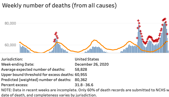
The apparent discrepancy November/December discrepancy between higher CovidTracking counts (COVID19 deaths) and lower CDC official excess death counts has essentially vanished.

The actual excess deaths amount to +6,500 per week for December. There was just a lot of lag.

I give myself some credit for considering that I might be in a bubble, that my faith in the two reporting systems might be too strong misplaced, and looking for alternate explanations.

But in the end I was too timid in their defense: I thought only about 5K of the 7K discrepancy would be lag, and that we would see a larger role of harvesting, for example.

Thanks to Mike Bishop for alerting me to Jiminez' 100-tweet thread and Lancet paper on the case for COVID-19 aerosols, and the fascinating 100-year history that still shapes debate.

Because of that history, it seems admitting “airborne” or “aerosol” has been quite a sea change. Some of this is important - “droplets” are supposed to drop, while aerosols remain airborne and so circulate farther.

But some seems definitional - a large enough aerosol is hindered by masks, and a small droplet doesn’t drop.

However, point being that like measles and other respiratory viruses, “miasma” isn’t a bad concept, so contagion can travel, esp. indoors.

VAERS Caveat

Please people, if using VAERS, go check the details. @RealJoeSmalley posts stuff like “9 child deaths in nearly 4,000 vaccinations”, but it’s not his responsibility if the data is wrong, caveat emptor.

With VAERS that’s highly irresponsible - you can’t even use VAERS without reading about its limits.

I get 9 deaths in VAERS if I set the limits to “<18”. But the number of total US vaccinations for <18 isn’t 4,000 - it’s 2.2M.

Also I checked the 9 VAERS deaths for <18:

Two are concerning because little/no risk:

5. 16yo, only risk factor oral contraceptives
6. 15yo, no known risks

Two+ are concerning but seem experimental. AFAIK the vaccines are not approved for breastfeeding, and are only in clinical trial for young children. Don’t try this at home:

2. 5mo breastmilk exposure - mom vaccinated. (?!)
3. 2yo in ¿illicit? trial? Very odd report saying it was a clinical trial but the doctors would deny that, reporter is untraceable, batch info is untraceable. Odd.
4. 1yo, seizure. (Clinical trial? Else how vaccinated?)

Two were very high risk patients. (Why was this even done?):

3. 15yo with about 25 severe pre-existing / allergies
4. 17yo w/~12 severe pre-existing / allergies

Two are clearly unrelated:

1. Error - gunshot suicide found by family, but age typed as “1.08”.
2. 17yo, firearm suicide - history of mental illness

For evaluating your risk, only the two teens would seem relevant. They might not be vaccine-related, but with otherwise no known risk, it’s a very good candidate cause.

VAERS Query

I’m not able to get “saved search” to work, so here’s the non-default Query Criteria:

• Age: < 6 months; 6-11 months; 1-2 years; 3-5 years; 6-17 years
• Event Category: Death
• Serious: Yes
• Vaccine Products: COVID19 VACCINE (COVID19)
• 
  

Group By: VAERS ID

An image of West Coast data science:

I keep climbing the leaderboard! … Life is pretty sweet. I pick up indoor rock climbing, sign up for wood working classes; I read Proust and books about espresso.

…Kaggle releases the final score. What an embarrassment! …Inevitably, I hike the Pacific Crest Trail and write a novel about it.

In competing w/o the data, a good discussion on fooling yourself using holdout sets.

Gelman’s recent short post on Relevance of Bad Science for Good Science includes a handy Top10 junk list:

A Ted talkin’ sleep researcher misrepresenting the literature or just plain making things up; a controversial sociologist drawing sexist conclusions from surveys of N=3000 where N=300,000 would be needed; a disgraced primatologist who wouldn’t share his data; a celebrity researcher in eating behavior who published purportedly empirical papers corresponding to no possible empirical data; an Excel error that may have influenced national economic policy; an iffy study that claimed to find that North Korea was more democratic than North Carolina; a claim, unsupported by data, that subliminal smiley faces could massively shift attitudes on immigration; various noise-shuffling statistical methods that just won’t go away—all of these, and more, represent different extremes of junk science.

And the following sobering reminder why we study failures:

None of us do all these things, and many of us try to do none of these things—but I think that most of us do some of these things much of the time.

CDC total deaths snapshot: December weekly #s gained about 4,500 vs. two weeks ago: there are now 4 weeks right near 80K, slightly above the highest April week.

That’s bad. But still hard to square with covidtracking deaths being 50% higher than in April.

Update 19-Feb

Week of 26-Dec is now at 81,406, up by ~1K. The week of 2-Jan is higher now, above 82K, gaining 1-2K.

#### Update 23-May

December totals are now about +26K versus April, or about +6,500/week. That’s pretty much all the discrepancy I was concerned to explain.

That further supports the live CovidTracking numbers from last autumn.

Bookmarking A methodology for agile data science by Edwin Thoen (ch.5 of Agile Data Science with R). Also favors Kanban. Highlights below.

As a rule of thumb, never work on more tasks simultaneously than the number of data scientists on the team.

One of the major pitfalls of trying to improve a data science product is endless exploration of a hypothesis.

How to manage exploration then?

The data scientist should not take longer for the task than the team agreed upfront, wrapping up even when he does not feel completely finished. If he found an alleyway that is still worthwhile exploring a new task should be put in the backlog, instead of persevering in the current task